3.1 Recursive Definitions

Predicates can be defined recursively. Roughly speaking, a predicate is recursively defined if one or more rules in its definition refers to itself.

Example 1: Eating

Consider the following knowledge base:

At first glance this seems pretty ordinary: it’s just a knowledge base containing three facts and two rules. But the definition of the is_digesting/2 predicate is recursive. Note that is_digesting/2 is (at least partially) defined in terms of itself, for the is_digesting/2 functor occurs in both the head and body of the second rule. Crucially, however, there is an ‘escape’ from this circularity. This is provided by the just_ate/2 predicate, which occurs in the first rule. (Significantly, the body of the first rule makes no mention of is_digesting/2 .) Let’s now consider both the declarative and procedural meanings of this definition.

The word “declarative” is used to talk about the logical meaning of Prolog knowledge bases. That is, the declarative meaning of a Prolog knowledge base is simply “what it says”, or “what it means, if we read it as a collection of logical statements”. And the declarative meaning of this recursive definition is fairly straightforward. The first clause (the escape clause, the one that is not recursive, or as we shall usually call it, the base clause), simply says that: if X has just eaten Y , then X is now digesting Y . This is obviously a sensible definition.

So what about the second clause, the recursive clause? This says that: if X has just eaten Z and Z is digesting Y , then X is digesting Y , too. Again, this is obviously a sensible definition.

So now we know what this recursive definition says, but what happens when we pose a query that actually needs to use this definition? That is, what does this definition actually do? To use the normal Prolog terminology, what is its procedural meaning?

This is also reasonably straightforward. The base rule is like all the earlier rules we’ve seen. That is, if we ask whether X is digesting Y , Prolog can use this rule to ask instead the question: has X just eaten Y ?

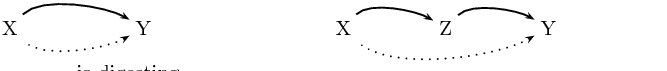
What about the recursive clause? This gives Prolog another strategy for determining whether X is digesting Y : it can try to find some Z such that X has just eaten Z , and Z is digesting Y . That is, this rule lets Prolog break the task apart into two subtasks. Hopefully, doing so will eventually lead to simple problems which can be solved by simply looking up the answers in the knowledge base. The following picture sums up the situation:

Let’s see how this works. If we pose the query:

then Prolog goes to work as follows. First, it tries to make use of the first rule listed concerning is_digesting ; that is, the base rule. This tells it that X is digesting Y if X just ate Y , By unifying X with stork and Y with mosquito it obtains the following goal:

But the knowledge base doesn’t contain the information that the stork just ate the mosquito, so this attempt fails. So Prolog next tries to make use of the second rule. By unifying X with stork and Y with mosquito it obtains the following goals:

That is, to show is_digesting(stork,mosquito) , Prolog needs to find a value for Z such that, firstly,

and secondly,

And there is such a value for Z , namely frog . It is immediate that

will succeed, for this fact is listed in the knowledge base. And deducing

is almost as simple, for the first clause of is_digesting/2 reduces this goal to deducing

and this is a fact listed in the knowledge base.

Well, that’s our first example of a recursive rule definition. We’re going to learn a lot more about them, but one very practical remark should be made right away. Hopefully it’s clear that when you write a recursive predicate, it should always have at least two clauses: a base clause (the clause that stops the recursion at some point), and one that contains the recursion. If you don’t do this, Prolog can spiral off into an unending sequence of useless computations. For example, here’s an extremely simple example of a recursive rule definition:

That’s it. Nothing else. It’s beautiful in its simplicity. And from a declarative perspective it’s an extremely sensible (if rather boring) definition: it says “if property p holds, then property p holds”. You can’t argue with that.

But from a procedural perspective, this is a wildly dangerous rule. In fact, we have here the ultimate in dangerous recursive rules: exactly the same thing on both sides, and no base clause to let us escape. For consider what happens when we pose the following query:

Prolog asks itself: “How do I prove p ?” and it realises, “Hey, I’ve got a rule for that! To prove p I just need to prove p !”. So it asks itself (again): “How do I prove p ?” and it realises, “Hey, I’ve got a rule for that! To prove p I just need to prove p !”. So it asks itself (yet again): “How do I prove p ?” and it realises, “Hey, I’ve got a rule for that! To prove p I just need to prove p !” and so on and so forth.

If you make this query, Prolog won’t answer you: it will head off, looping desperately away in an unending search. That is, it won’t terminate, and you’ll have to interrupt it. Of course, if you use trace , you can step through one step at a time, until you get sick of watching Prolog loop.

Example 2: Descendant

Now that we know something about what recursion in Prolog involves, it is time to ask why it is so important. Actually, this is a question that can be answered on a number of levels, but for now, let’s keep things fairly practical. So: when it comes to writing useful Prolog programs, are recursive definitions really so important? And if so, why?

Let’s consider an example. Suppose we have a knowledge base recording facts about the child relation:

That is, Caroline is a child of Bridget, and Donna is a child of Caroline. Now suppose we wished to define the descendant relation; that is, the relation of being a child of, or a child of a child of, or a child of a child of a child of, and so on. Here’s a first attempt to do this. We could add the following two non -recursive rules to the knowledge base:

Now, fairly obviously these definitions work up to a point, but they are clearly limited: they only define the concept of descendant-of for two generations or less. That’s ok for the above knowledge base, but suppose we get some more information about the child-of relation and we expand our list of child-of facts to this:

Now our two rules are inadequate. For example, if we pose the queries

or

we get the answer no, which is not what we want. Sure, we could ‘fix’ this by adding the following two rules:

But, let’s face it, this is clumsy and hard to read. Moreover, if we add further child-of facts, we could easily find ourselves having to add more and more rules as our list of child-of facts grow, rules like:

This is not a particularly pleasant (or sensible) way to go!

But we don’t need to do this at all. We can avoid having to use ever longer rules entirely. The following recursive predicate definition fixes everything exactly the way we want:

What does this say? The declarative meaning of the base clause is: if Y is a child of X , then Y is a descendant of X . Obviously sensible. So what about the recursive clause? Its declarative meaning is: if Z is a child of X , and Y is a descendant of Z , then Y is a descendant of X . Again, this is obviously true.

So let’s now look at the procedural meaning of this recursive predicate, by stepping through an example. What happens when we pose the query:

Prolog first tries the first rule. The variable X in the head of the rule is unified with anne and Y with donna and the next goal Prolog tries to prove is

This attempt fails, however, since the knowledge base neither contains the fact child(anne,donna) nor any rules that would allow to infer it. So Prolog backtracks and looks for an alternative way of proving descend(anne,donna) . It finds the second rule in the knowledge base and now has the following subgoals:

Prolog takes the first subgoal and tries to unify it with something in the knowledge base. It finds the fact child(anne,bridget) and the variable _633 gets instantiated to bridget . Now that the first subgoal is satisfied, Prolog moves to the second subgoal. It has to prove

This is the first recursive call of the predicate descend/2 . As before, Prolog starts with the first rule, but fails, because the goal

cannot be proved. Backtracking, Prolog finds that there is a second possibility to be checked for descend(bridget,donna) , namely the second rule, which again gives Prolog two new subgoals:

The first one can be unified with the fact child(bridget,caroline) of the knowledge base, so that the variable _1785 is instantiated with caroline . Next Prolog tries to prove

This is the second recursive call of predicate descend/2 . As before, it tries the first rule first, obtaining the following new goal:

This time Prolog succeeds, since child(caroline,donna) is a fact in the database. Prolog has found a proof for the goal descend(caroline,donna) (the second recursive call). But this means that descend(bridget,donna) (the first recursive call) is also true, which means that our original query descend(anne,donna) is true as well.

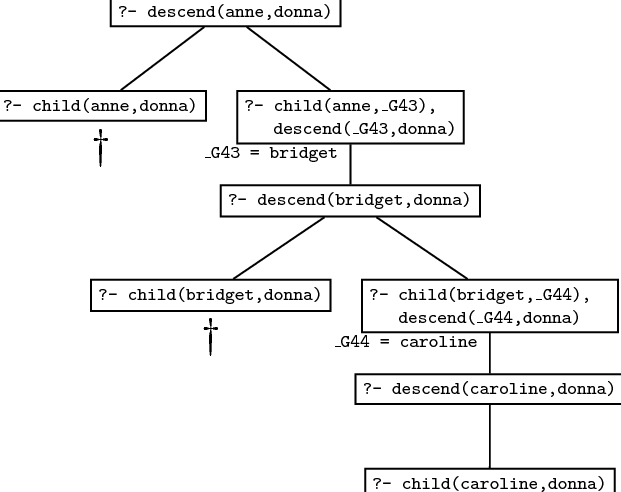
Here is the search tree for the query descend(anne,donna) . Make sure that you understand how it relates to the discussion in the text; that is, how Prolog traverses this search tree when trying to prove this query.

It should be obvious from this example that no matter how many generations of children we add, we will always be able to work out the descendant relation. That is, the recursive definition is both general and compact: it contains all the information in the non-recursive rules, and much more besides. The non-recursive rules only defined the descendant concept up to some fixed number of generations: we would need to write down infinitely many non-recursive rules if we wanted to capture this concept fully, and of course that’s impossible. But, in effect, that’s what the recursive rule does for us: it bundles up the information needed to cope with arbitrary numbers of generations into just three lines of code.

Recursive rules are really important. They enable to pack an enormous amount of information into a compact form and to define predicates in a natural way. Most of the work you will do as a Prolog programmer will involve writing recursive rules.

Example 3: Successor

In the previous chapter we remarked that building structure through unification is a key idea in Prolog programming. Now that we know about recursion, we can give more interesting illustrations of this.

Nowadays, when human beings write numerals, they usually use decimal notation (0, 1, 2, 3, 4, 5, 6, 7, 8, 9, 10, 11, 12, and so on) but as you probably know, there are many other notations. For example, because computer hardware is generally based on digital circuits, computers usually use binary notation to represent numerals (0, 1, 10, 11, 100, 101, 110, 111, 1000, and so on), for the 0 can be implemented as a switch being off, the 1 as a switch being on. Other cultures use different systems. For example, the ancient Babylonians used a base 60 system, while the ancient Romans used a rather ad-hoc system (I, II, III, IV, V, VI, VII, VIII, IX, X). This last example shows that notational issues can be important. If you don’t believe this, try figuring out a systematic way of doing long-division in Roman notation. As you’ll discover, it’s a frustrating task. Apparently the Romans had a group of professionals (analogs of modern accountants) who specialised in this.

Well, here’s yet another way of writing numerals, which is sometimes used in mathematical logic. It makes use of just four symbols: 0, succ , and the left and right parentheses. This style of numeral is defined by the following inductive definition:

1. 0 is a numeral.
2. If X is a numeral, then so is succ(X) .

As is probably clear, succ can be read as short for successor . That is, succ(X) represents the number obtained by adding one to the number represented by X . So this is a very simple notation: it simply says that 0 is a numeral, and that all other numerals are built by stacking succ symbols in front. (In fact, it’s used in mathematical logic because of this simplicity. Although it wouldn’t be pleasant to do household accounts in this notation, it is a very easy notation to prove things about .)

Now, by this stage it should be clear that we can turn this definition into a Prolog program. The following knowledge base does this:

So if we pose queries like

we get the answer yes.

But we can do some more interesting things. Consider what happens when we pose the following query:

That is, we’re saying “Ok, show me some numerals”. Then we can have the following dialogue with Prolog:

Yes, Prolog is counting: but what’s really important is how it’s doing this. Quite simply, it’s backtracking through the recursive definition, and actually building numerals using unification. This is an instructive example, and it is important that you understand it. The best way to do so is to sit down and try it out, with trace turned on.

Building and binding. Recursion, unification, and proof search. These are ideas that lie at the heart of Prolog programming. Whenever we have to generate or analyse recursively structured objects (such as these numerals) the interplay of these ideas makes Prolog a powerful tool. For example, in the next chapter we shall introduce lists, an extremely important recursive data structure, and we will see that Prolog is a natural list processing language. Many applications (computational linguistics is a prime example) make heavy use of recursively structured objects, such as trees and feature structures. So it’s not particularly surprising that Prolog has proved useful in such applications.

Example 4: Addition

As a final example, let’s see whether we can use the representation of numerals that we introduced in the previous section for doing simple arithmetic. Let’s try to define addition. That is, we want to define a predicate add/3 which when given two numerals as the first and second argument returns the result of adding them up as its third argument. For example:

There are two things which are important to notice:

1. Whenever the first argument is 0 , the third argument has to be the same as the second argument:
      ?-  add(0,succ(succ(0)),Y).
      Y  =  succ(succ(0))
      ?-  add(0,0,Y).
      Y  =  0

   This is the case that we want to use for the base clause.

2. Assume that we want to add the two numerals X and Y (for example succ(succ(succ(0))) and succ(succ(0)) ) and that X is not 0 . Now, if X1 is the numeral that has one succ functor less than X (that is, succ(succ(0)) in our example) and if we know the result – let’s call it Z – of adding X1 and Y (namely succ(succ(succ(succ(0)))) ), then it is very easy to compute the result of adding X and Y : we just have to add one succ -functor to Z . This is what we want to express with the recursive clause.

Here is the predicate definition that expresses exactly what we just said:

So what happens, if we give Prolog this predicate definition and then ask:

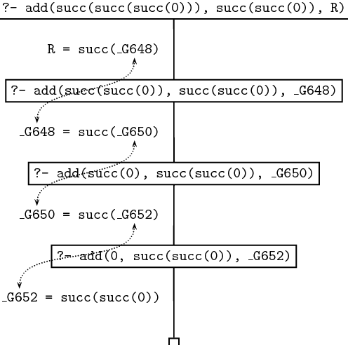
Let’s go step by step through the way Prolog processes this query. The trace and search tree for the query are given below.

The first argument is not 0 , which means that only the second clause for add/3 can be used. This leads to a recursive call of add/3 . The outermost succ functor is stripped off the first argument of the original query, and the result becomes the first argument of the recursive query. The second argument is passed on unchanged to the recursive query, and the third argument of the recursive query is a variable, the internal variable _G648 in the trace given below. Note that _G648 is not instantiated yet. However it shares values with R (the variable that we used as the third argument in the original query) because R was instantiated to succ(_G648) when the query was unified with the head of the second clause. But that means that R is not a completely uninstantiated variable anymore. It is now a complex term, that has a (uninstantiated) variable as its argument.

The next two steps are essentially the same. With every step the first argument becomes one layer of succ smaller; both the trace and the search tree given below show this nicely. At the same time, a succ functor is added to R at every step, but always leaving the innermost variable uninstantiated. After the first recursive call R is succ(_G648) . After the second recursive call, _G648 is instantiated with succ(_G650) , so that R is succ(succ(_G650) . After the third recursive call, _G650 is instantiated with succ(_G652) and R therefore becomes succ(succ(succ(_G652))) . The search tree shows this step by step instantiation.

At this stage all succ functors have been stripped off the first argument and we can apply the base clause. The third argument is equated with the second argument, so the ‘hole’ (the uninstantiated variable) in the complex term R is finally filled, and we are through.

Here’s the complete trace of our query:

And here’s the search tree: