2.2 Proof Search

Now that we know about unification, we are in a position to learn how Prolog actually searches a knowledge base to see if a query is satisfied. That is, we are ready to learn about proof search. We will introduce the basic ideas involved by working through a simple example.

Suppose we are working with the following knowledge base

Suppose we then pose the query

It is probably clear that there is only one answer to this query, namely k(b) , but how exactly does Prolog work this out? Let’s see.

Prolog reads the knowledge base, and tries to unify k(Y) with either a fact, or the head of a rule. It searches the knowledge base top to bottom, and carries out the unification, if it can, at the first place possible. Here there is only one possibility: it must unify k(Y) to the head of the rule k(X)  :-  f(X),  g(X),  h(X) .

When Prolog unifies the variable in a query to a variable in a fact or rule, it generates a brand new variable (say _G34 ) to represent the shared variables. So the original query now reads:

and Prolog knows that

So what do we now have? The original query says: “I want to find an individual that has property k ”. The rule says, “an individual has property k if it has properties f , g , and h ”. So if Prolog can find an individual with properties f , g , and h , it will have satisfied the original query. So Prolog replaces the original query with the following list of goals:

Our discussion of the querying process so far can be made more elegant and succinct if we think graphically. Consider the following diagram:

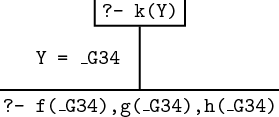
Everything in a box is either a query or a goal. In particular, our original goal was to prove k(Y) , thus this is shown in the top box. When we unified k(Y) with the head of the rule in the knowledge base, X Y , and the new internal variable _G34 were made to share values, and we were left with the goals f(_G34),g(_G34),h(_G34) , just as shown.

Now, whenever it has a list of goals, Prolog tries to satisfy them one by one, working through the list in a left to right direction. The leftmost goal is f(_G34) , which reads: “I want an individual with property f ”. Can this goal be satisfied? Prolog tries to do so by searching through the knowledge base from top to bottom. The first item it finds that unifies with this goal is the fact f(a) . This satisfies the goal f(_G34) and we are left with two more goals. Now, when we unify f(_G34) to f(a) , _G34 is instantiated to a , and this instantiation applies to all occurrences of _G34 in the list of goals. So the list now looks like this:

and our graphical representation of the proof search now looks like this:

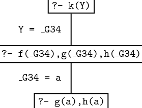
But the fact g(a) is in the knowledge base, so the first goal we have to prove is satisfied too. So the goal list becomes

and the graphical representation is now

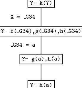
But there is no way to satisfy h(a) , the last remaining goal. The only information about h we have in the knowledge base is h(b) , and this won’t unify with h(a) .

So what happens next? Well, Prolog decides it has made a mistake, and checks whether it has missed any possible ways of unifying a goal with a fact or the head of a rule in the knowledge base. It does this by going back up the path shown in the graphical representation, looking for alternatives. Now, there is nothing else in the knowledge base that unifies with g(a) , but there is another way of unifying f(_G34) . Points in the search where there are several alternative ways of unifying a goal against the knowledge base are called choice points. Prolog keeps track of choice points it has encountered, so that if it makes a wrong choice it can retreat to the previous choice point and try something else instead. This process is called backtracking, and it is fundamental to proof search in Prolog.

So let’s carry on with our example. Prolog backtracks to the last choice point. This is the point in the graphical representation where the list of goals was:

Prolog must now redo this work. First it must try to re-satisfy the first goal by searching further in the knowledge base. It can do this: it sees that it can unify the first goal with information in the knowledge base by unifying f(_G34) with f(b) . This satisfies the goal f(_G34) and instantiates X to b , so that the remaining goal list is

But g(b) is a fact in the knowledge base, so this is satisfied too, leaving the goal list:

Moreover, this fact too is in the knowledge base, so this goal is also satisfied. So Prolog now has an empty list of goals. This means that it has now proved everything required to establish the original goal (that is, k(Y) ). So the original query is satisfiable, and moreover, Prolog has also discovered what it has to do to satisfy it (namely instantiate Y to b ).

It is interesting to consider what happens if we then ask for another solution by typing:

This forces Prolog to backtrack to the last choice point, to try and find another possibility. However, there are no other choice points, as there are no other possibilities for unifying h(b) , g(b) , f(_G34) , or k(Y) with clauses in the knowledge base, so Prolog would respond no. On the other hand, if there had been other rules involving k , Prolog would have gone off and tried to use them in exactly the way we have described: that is, by searching top to bottom in the knowledge base, left to right in goal lists, and backtracking to the previous choice point whenever it fails.

Let’s take a look at the graphical representation of the entire search process. Some general remarks are called for, for such representations are an important way of thinking about proof search in Prolog.

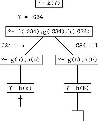
This diagram has the form of a tree; in fact it is our first example of what is known as a search tree. The nodes of such trees say which goals have to be satisfied at the various steps of the proof search, and the edges keep track of the variable instantiations that are made when the current goal (that is, the first one in the list of goals) is unified to a fact or to the head of a rule in the knowledge base. Leaf nodes which still contain unsatisfied goals are points where Prolog failed (either because it made a wrong decision somewhere along the path, or because no solution exists). Leaf nodes with an empty goal list correspond to a possible solution. The edges along the path from the root node to a successful leaf node tell you the variable instantiations that need to be made to satisfy the original query.

Let’s have a look at another example. Suppose that we are working with the following knowledge base:

Now we pose the query

The search tree for the query looks like this:

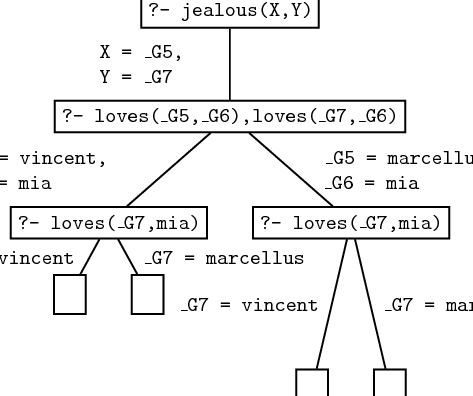
There is only one possible way of unifying jealous(X,Y) against the knowledge base, namely by using the rule

So the new goals that have to be satisfied are:

Now we have to unify loves(_G5,_G6) against the knowledge base. There are two ways of doing this (it can either be unified with the first fact or with the second fact) and this is why the path branches at this point. In both cases the goal loves(_G7,mia) remains, and this can also be satisfied by using either of two facts. All in all there are four leaf nodes with an empty goal list, which means that there are four ways of satisfying the original query. The variable instantiations for each solution can be read off the path from the root to the leaf node. So the four solutions are:

1. X  =  _G5  =  vincent and Y  =  _G7  =  vincent
2. X  =  _G5  =  vincent and Y  =  _G7  =  marcellus
3. X  =  _G5  =  marcellus and Y  =  _G7  =  vincent
4. X  =  _G5  =  marcellus and Y  =  _G7  =  marcellus

Work through this example carefully, and make sure you understand it.